Implementing Logistic Regression for Predicting if a Tumor is Malignant or Benign (From Scratch)

Introduction

Bellow is my notebook from Kaggle for my project on implementing Logistic Regression from scratch for Predicting if a Tumor is Malignant or Benign and comparing it to scikit-learn predefined one.
Enjoy!

Notebook

# This Python 3 environment comes with many helpful analytics libraries installed
# It is defined by the kaggle/python Docker image: https://github.com/kaggle/docker-python
# For example, here's several helpful packages to load

import numpy as np # linear algebra
import pandas as pd # data processing, CSV file I/O (e.g. pd.read_csv)

# Input data files are available in the read-only "../input/" directory
# For example, running this (by clicking run or pressing Shift+Enter) will list all files under the input directory

import os
for dirname, _, filenames in os.walk('/kaggle/input'):
    for filename in filenames:
        print(os.path.join(dirname, filename))

# You can write up to 20GB to the current directory (/kaggle/working/) that gets preserved as output when you create a version using "Save & Run All" 
# You can also write temporary files to /kaggle/temp/, but they won't be saved outside of the current session

/kaggle/input/breast-cancer-wisconsin-data/data.csv

Overview

In this notebook i will predict if a Tumor is Malignant or Benign using logistic regression. i will implement everything from scratch then compare my results to a predefined algorithm in scikit learn.

Dataset

first i will load and explore the dataset. i’m working on Breast Cancer Wisconsin (Diagnostic) Data Set on Kaggle

https://www.kaggle.com/datasets/uciml/breast-cancer-wisconsin-data

df = pd.read_csv("/kaggle/input/breast-cancer-wisconsin-data/data.csv")
df.head()

	id	diagnosis	radius_mean	texture_mean	perimeter_mean	area_mean	smoothness_mean	compactness_mean	concavity_mean	concave points_mean	...	texture_worst	perimeter_worst	area_worst	smoothness_worst	compactness_worst	concavity_worst	concave points_worst	symmetry_worst	fractal_dimension_worst	Unnamed: 32
0	842302	M	17.99	10.38	122.80	1001.0	0.11840	0.27760	0.3001	0.14710	...	17.33	184.60	2019.0	0.1622	0.6656	0.7119	0.2654	0.4601	0.11890	NaN
1	842517	M	20.57	17.77	132.90	1326.0	0.08474	0.07864	0.0869	0.07017	...	23.41	158.80	1956.0	0.1238	0.1866	0.2416	0.1860	0.2750	0.08902	NaN
2	84300903	M	19.69	21.25	130.00	1203.0	0.10960	0.15990	0.1974	0.12790	...	25.53	152.50	1709.0	0.1444	0.4245	0.4504	0.2430	0.3613	0.08758	NaN
3	84348301	M	11.42	20.38	77.58	386.1	0.14250	0.28390	0.2414	0.10520	...	26.50	98.87	567.7	0.2098	0.8663	0.6869	0.2575	0.6638	0.17300	NaN
4	84358402	M	20.29	14.34	135.10	1297.0	0.10030	0.13280	0.1980	0.10430	...	16.67	152.20	1575.0	0.1374	0.2050	0.4000	0.1625	0.2364	0.07678	NaN

5 rows × 33 columns

df.shape

(569, 33)

df.info()

<class 'pandas.core.frame.DataFrame'>
RangeIndex: 569 entries, 0 to 568
Data columns (total 33 columns):
 #   Column                   Non-Null Count  Dtype  
---  ------                   --------------  -----  
 0   id                       569 non-null    int64  
 1   diagnosis                569 non-null    object 
 2   radius_mean              569 non-null    float64
 3   texture_mean             569 non-null    float64
 4   perimeter_mean           569 non-null    float64
 5   area_mean                569 non-null    float64
 6   smoothness_mean          569 non-null    float64
 7   compactness_mean         569 non-null    float64
 8   concavity_mean           569 non-null    float64
 9   concave points_mean      569 non-null    float64
 10  symmetry_mean            569 non-null    float64
 11  fractal_dimension_mean   569 non-null    float64
 12  radius_se                569 non-null    float64
 13  texture_se               569 non-null    float64
 14  perimeter_se             569 non-null    float64
 15  area_se                  569 non-null    float64
 16  smoothness_se            569 non-null    float64
 17  compactness_se           569 non-null    float64
 18  concavity_se             569 non-null    float64
 19  concave points_se        569 non-null    float64
 20  symmetry_se              569 non-null    float64
 21  fractal_dimension_se     569 non-null    float64
 22  radius_worst             569 non-null    float64
 23  texture_worst            569 non-null    float64
 24  perimeter_worst          569 non-null    float64
 25  area_worst               569 non-null    float64
 26  smoothness_worst         569 non-null    float64
 27  compactness_worst        569 non-null    float64
 28  concavity_worst          569 non-null    float64
 29  concave points_worst     569 non-null    float64
 30  symmetry_worst           569 non-null    float64
 31  fractal_dimension_worst  569 non-null    float64
 32  Unnamed: 32              0 non-null      float64
dtypes: float64(31), int64(1), object(1)
memory usage: 146.8+ KB

df.describe()

	id	radius_mean	texture_mean	perimeter_mean	area_mean	smoothness_mean	compactness_mean	concavity_mean	concave points_mean	symmetry_mean	...	texture_worst	perimeter_worst	area_worst	smoothness_worst	compactness_worst	concavity_worst	concave points_worst	symmetry_worst	fractal_dimension_worst	Unnamed: 32
count	5.690000e+02	569.000000	569.000000	569.000000	569.000000	569.000000	569.000000	569.000000	569.000000	569.000000	...	569.000000	569.000000	569.000000	569.000000	569.000000	569.000000	569.000000	569.000000	569.000000	0.0
mean	3.037183e+07	14.127292	19.289649	91.969033	654.889104	0.096360	0.104341	0.088799	0.048919	0.181162	...	25.677223	107.261213	880.583128	0.132369	0.254265	0.272188	0.114606	0.290076	0.083946	NaN
std	1.250206e+08	3.524049	4.301036	24.298981	351.914129	0.014064	0.052813	0.079720	0.038803	0.027414	...	6.146258	33.602542	569.356993	0.022832	0.157336	0.208624	0.065732	0.061867	0.018061	NaN
min	8.670000e+03	6.981000	9.710000	43.790000	143.500000	0.052630	0.019380	0.000000	0.000000	0.106000	...	12.020000	50.410000	185.200000	0.071170	0.027290	0.000000	0.000000	0.156500	0.055040	NaN
25%	8.692180e+05	11.700000	16.170000	75.170000	420.300000	0.086370	0.064920	0.029560	0.020310	0.161900	...	21.080000	84.110000	515.300000	0.116600	0.147200	0.114500	0.064930	0.250400	0.071460	NaN
50%	9.060240e+05	13.370000	18.840000	86.240000	551.100000	0.095870	0.092630	0.061540	0.033500	0.179200	...	25.410000	97.660000	686.500000	0.131300	0.211900	0.226700	0.099930	0.282200	0.080040	NaN
75%	8.813129e+06	15.780000	21.800000	104.100000	782.700000	0.105300	0.130400	0.130700	0.074000	0.195700	...	29.720000	125.400000	1084.000000	0.146000	0.339100	0.382900	0.161400	0.317900	0.092080	NaN
max	9.113205e+08	28.110000	39.280000	188.500000	2501.000000	0.163400	0.345400	0.426800	0.201200	0.304000	...	49.540000	251.200000	4254.000000	0.222600	1.058000	1.252000	0.291000	0.663800	0.207500	NaN

8 rows × 32 columns

list(df.columns.values)

['id',
 'diagnosis',
 'radius_mean',
 'texture_mean',
 'perimeter_mean',
 'area_mean',
 'smoothness_mean',
 'compactness_mean',
 'concavity_mean',
 'concave points_mean',
 'symmetry_mean',
 'fractal_dimension_mean',
 'radius_se',
 'texture_se',
 'perimeter_se',
 'area_se',
 'smoothness_se',
 'compactness_se',
 'concavity_se',
 'concave points_se',
 'symmetry_se',
 'fractal_dimension_se',
 'radius_worst',
 'texture_worst',
 'perimeter_worst',
 'area_worst',
 'smoothness_worst',
 'compactness_worst',
 'concavity_worst',
 'concave points_worst',
 'symmetry_worst',
 'fractal_dimension_worst',
 'Unnamed: 32']

Here i noticed a column named ‘Unnamed: 32’ and there values are NaN

df.drop(["Unnamed: 32"], axis = 1, inplace=True)
list(df.columns.values)

['id',
 'diagnosis',
 'radius_mean',
 'texture_mean',
 'perimeter_mean',
 'area_mean',
 'smoothness_mean',
 'compactness_mean',
 'concavity_mean',
 'concave points_mean',
 'symmetry_mean',
 'fractal_dimension_mean',
 'radius_se',
 'texture_se',
 'perimeter_se',
 'area_se',
 'smoothness_se',
 'compactness_se',
 'concavity_se',
 'concave points_se',
 'symmetry_se',
 'fractal_dimension_se',
 'radius_worst',
 'texture_worst',
 'perimeter_worst',
 'area_worst',
 'smoothness_worst',
 'compactness_worst',
 'concavity_worst',
 'concave points_worst',
 'symmetry_worst',
 'fractal_dimension_worst']

Now we are talking :)

# Shuffle the data
data = df.sample(frac=1, random_state=42).reset_index(drop=True)

# Calculate the number of samples for each set
train_size = int(0.8 * len(data))
test_size = int(0.2 * len(data))

# Split the dataset into training and test sets
train_data = data[:train_size] # training data (80%)
test_data = data[train_size:] # test data (20%)

# Split the features and target for each set
X_train = train_data.drop('diagnosis', axis=1)
y_train = train_data['diagnosis']

X_test = test_data.drop('diagnosis', axis=1)
y_test = test_data['diagnosis']

y_train = y_train.map({'M': 1, 'B': 0}).astype(np.float64)
y_test = y_test.map({'M': 1, 'B': 0}).astype(np.float64)

print(f"Training set size: {len(X_train)} samples")
print(f"Test set size: {len(X_test)} samples")

Training set size: 455 samples
Test set size: 114 samples

Models

Logistic Regression from scratch

import matplotlib.pyplot as plt

class LogisticRegression :
    def __init__(self, alpha=0.01, iterations=1000, scale=False):
        self.alpha = alpha
        self.iterations = iterations
        self.scale = scale
        self.w = None
        self.b = None
        self.cost_history = []

    def scale_features(self,X):
        """Scale features using mean and std deviation (standardization)."""
        self.mean = np.mean(X, axis=0)
        self.std = np.std(X, axis=0)
        return (X - self.mean) / self.std


    def fit(self, X, y):
        m = len(y) # Number of training examples

        # Scale the features if needed
        if self.scale : 
            X = self.scale_features(X)
        
        # Initialize weights and bias
        self.w = np.zeros(X.shape[1])
        self.b = 0
        
        for i in range(self.iterations):
            
            z = X.dot(self.w) + self.b
            # pred = np.where(z >= 0, 1 / (1 + np.exp(-z)), np.exp(z) / (1 + np.exp(z)))
            pred = 1 / (1 + np.exp(-z))
            
            epsilon = 1e-8
            pred = np.clip(pred, epsilon, 1 - epsilon)
            
            error = pred - y

            dw = (1/m) * np.dot(X.T , error)
            db = (1/m) * np.sum(error)

            # Update the weights and bias
            self.w -= self.alpha * dw
            self.b -= self.alpha * db

            # Calculate and store the cost
            cost = (-1/m) * np.sum(y * np.log(pred) + (1 - y) * np.log(1 - pred))
            self.cost_history.append(cost)

    def predict(self,X):
        """Make predictions using the trained model."""
        if self.scale:
            X = (X - self.mean) / self.std
        logits = X.dot(self.w) + self.b
        prob = 1 / (1 + np.exp(-logits))
        return (prob >= 0.5).astype(int)

    def predict_proba(self, X):
        """Return probability estimates for the positive class."""
        if self.scale:
            X = (X - self.mean) / self.std
        logits = X.dot(self.w) + self.b
        return 1 / (1 + np.exp(-logits))

    def get_cost_history(self):
        return self.cost_history

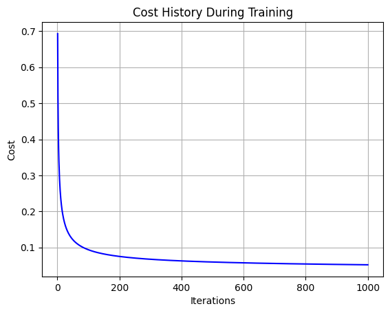
# Initialize and train the model
model = LogisticRegression(alpha=0.1, iterations=1000, scale=True)
model.fit(X_train, y_train)

cost_history = model.get_cost_history()

plt.plot(range(1, len(cost_history) + 1), cost_history, color='blue')
plt.title('Cost History During Training')
plt.xlabel('Iterations')
plt.ylabel('Cost')
plt.grid(True)
plt.show()

# Make predictions on all datasets
y_train_pred = model.predict(X_train)
y_test_pred = model.predict(X_test)

from sklearn.metrics import accuracy_score
from sklearn.metrics import confusion_matrix
from sklearn.metrics import classification_report
from sklearn.metrics import roc_auc_score, roc_curve

train_accuracy = accuracy_score(y_train, y_train_pred)
test_accuracy = accuracy_score(y_test, y_test_pred)

print(f"Training Accuracy: {train_accuracy}")
print(f"Test Accuracy: {test_accuracy}")

conf_matrix = confusion_matrix(y_test, y_test_pred)
print("Confusion Matrix:")
print(conf_matrix)

report = classification_report(y_test, y_test_pred)
print("Classification Report:")
print(report)

Training Accuracy: 0.9912087912087912
Test Accuracy: 0.9736842105263158
Confusion Matrix:
[[66  1]
 [ 2 45]]
Classification Report:
              precision    recall  f1-score   support

         0.0       0.97      0.99      0.98        67
         1.0       0.98      0.96      0.97        47

    accuracy                           0.97       114
   macro avg       0.97      0.97      0.97       114
weighted avg       0.97      0.97      0.97       114

Logistic Regression using scikit-learn

from sklearn.linear_model import LogisticRegression as SklearnLogisticRegression
from sklearn.preprocessing import StandardScaler

# Scale the features
scaler = StandardScaler()
X_train_scaled = scaler.fit_transform(X_train)
X_test_scaled = scaler.transform(X_test)

# Initialize and train the sklearn logistic regression model
clf = SklearnLogisticRegression(random_state=42, solver='lbfgs', max_iter=1000)
clf.fit(X_train_scaled, y_train)

# Make predictions on the training and test sets
y_train_pred_sklearn = clf.predict(X_train_scaled)
y_test_pred_sklearn = clf.predict(X_test_scaled)

# Evaluate the performance
train_accuracy = accuracy_score(y_train, y_train_pred_sklearn)
test_accuracy = accuracy_score(y_test, y_test_pred_sklearn)
conf_matrix = confusion_matrix(y_test, y_test_pred_sklearn)
class_report = classification_report(y_test, y_test_pred_sklearn)

print("Training Accuracy:", train_accuracy)
print("Test Accuracy:", test_accuracy)
print("Confusion Matrix:")
print(conf_matrix)
print("Classification Report:")
print(class_report)

Training Accuracy: 0.9934065934065934
Test Accuracy: 0.956140350877193
Confusion Matrix:
[[66  1]
 [ 4 43]]
Classification Report:
              precision    recall  f1-score   support

         0.0       0.94      0.99      0.96        67
         1.0       0.98      0.91      0.95        47

    accuracy                           0.96       114
   macro avg       0.96      0.95      0.95       114
weighted avg       0.96      0.96      0.96       114