Implementing Polynomial Regression for Predicting Car Price (From Scratch)

Introduction

Bellow is my notebook from Kaggle for my project on implementing Polynomial Regression from scratch for Predicting Car Price and comparing it to scikit-learn predefined one.
Enjoy!

Notebook

# This Python 3 environment comes with many helpful analytics libraries installed
# It is defined by the kaggle/python Docker image: https://github.com/kaggle/docker-python
# For example, here's several helpful packages to load

import numpy as np # linear algebra
import pandas as pd # data processing, CSV file I/O (e.g. pd.read_csv)

# Input data files are available in the read-only "../input/" directory
# For example, running this (by clicking run or pressing Shift+Enter) will list all files under the input directory

import os
for dirname, _, filenames in os.walk('/kaggle/input'):
    for filename in filenames:
        print(os.path.join(dirname, filename))

# You can write up to 20GB to the current directory (/kaggle/working/) that gets preserved as output when you create a version using "Save & Run All" 
# You can also write temporary files to /kaggle/temp/, but they won't be saved outside of the current session

/kaggle/input/car-price-prediction/CarPrice_Assignment.csv
/kaggle/input/car-price-prediction/Data Dictionary - carprices.xlsx

Overview

In this notebook i will predict Car Price using polynomial regression. i will implement everything from scratch then compare my results to a predefined algorithm in scikit learn.

Dataset

first i will load and explore the dataset. i’m working on Car Price Prediction Data Set on Kaggle

https://www.kaggle.com/datasets/hellbuoy/car-price-prediction

df = pd.read_csv("/kaggle/input/car-price-prediction/CarPrice_Assignment.csv")
df.head()

	car_ID	symboling	CarName	fueltype	aspiration	doornumber	carbody	drivewheel	enginelocation	wheelbase	...	enginesize	fuelsystem	boreratio	stroke	compressionratio	horsepower	peakrpm	citympg	highwaympg	price
0	1	3	alfa-romero giulia	gas	std	two	convertible	rwd	front	88.6	...	130	mpfi	3.47	2.68	9.0	111	5000	21	27	13495.0
1	2	3	alfa-romero stelvio	gas	std	two	convertible	rwd	front	88.6	...	130	mpfi	3.47	2.68	9.0	111	5000	21	27	16500.0
2	3	1	alfa-romero Quadrifoglio	gas	std	two	hatchback	rwd	front	94.5	...	152	mpfi	2.68	3.47	9.0	154	5000	19	26	16500.0
3	4	2	audi 100 ls	gas	std	four	sedan	fwd	front	99.8	...	109	mpfi	3.19	3.40	10.0	102	5500	24	30	13950.0
4	5	2	audi 100ls	gas	std	four	sedan	4wd	front	99.4	...	136	mpfi	3.19	3.40	8.0	115	5500	18	22	17450.0

5 rows × 26 columns

df.shape

(205, 26)

df.info()

<class 'pandas.core.frame.DataFrame'>
RangeIndex: 205 entries, 0 to 204
Data columns (total 26 columns):
 #   Column            Non-Null Count  Dtype  
---  ------            --------------  -----  
 0   car_ID            205 non-null    int64  
 1   symboling         205 non-null    int64  
 2   CarName           205 non-null    object 
 3   fueltype          205 non-null    object 
 4   aspiration        205 non-null    object 
 5   doornumber        205 non-null    object 
 6   carbody           205 non-null    object 
 7   drivewheel        205 non-null    object 
 8   enginelocation    205 non-null    object 
 9   wheelbase         205 non-null    float64
 10  carlength         205 non-null    float64
 11  carwidth          205 non-null    float64
 12  carheight         205 non-null    float64
 13  curbweight        205 non-null    int64  
 14  enginetype        205 non-null    object 
 15  cylindernumber    205 non-null    object 
 16  enginesize        205 non-null    int64  
 17  fuelsystem        205 non-null    object 
 18  boreratio         205 non-null    float64
 19  stroke            205 non-null    float64
 20  compressionratio  205 non-null    float64
 21  horsepower        205 non-null    int64  
 22  peakrpm           205 non-null    int64  
 23  citympg           205 non-null    int64  
 24  highwaympg        205 non-null    int64  
 25  price             205 non-null    float64
dtypes: float64(8), int64(8), object(10)
memory usage: 41.8+ KB

df.describe()

	car_ID	symboling	wheelbase	carlength	carwidth	carheight	curbweight	enginesize	boreratio	stroke	compressionratio	horsepower	peakrpm	citympg	highwaympg	price
count	205.000000	205.000000	205.000000	205.000000	205.000000	205.000000	205.000000	205.000000	205.000000	205.000000	205.000000	205.000000	205.000000	205.000000	205.000000	205.000000
mean	103.000000	0.834146	98.756585	174.049268	65.907805	53.724878	2555.565854	126.907317	3.329756	3.255415	10.142537	104.117073	5125.121951	25.219512	30.751220	13276.710571
std	59.322565	1.245307	6.021776	12.337289	2.145204	2.443522	520.680204	41.642693	0.270844	0.313597	3.972040	39.544167	476.985643	6.542142	6.886443	7988.852332
min	1.000000	-2.000000	86.600000	141.100000	60.300000	47.800000	1488.000000	61.000000	2.540000	2.070000	7.000000	48.000000	4150.000000	13.000000	16.000000	5118.000000
25%	52.000000	0.000000	94.500000	166.300000	64.100000	52.000000	2145.000000	97.000000	3.150000	3.110000	8.600000	70.000000	4800.000000	19.000000	25.000000	7788.000000
50%	103.000000	1.000000	97.000000	173.200000	65.500000	54.100000	2414.000000	120.000000	3.310000	3.290000	9.000000	95.000000	5200.000000	24.000000	30.000000	10295.000000
75%	154.000000	2.000000	102.400000	183.100000	66.900000	55.500000	2935.000000	141.000000	3.580000	3.410000	9.400000	116.000000	5500.000000	30.000000	34.000000	16503.000000
max	205.000000	3.000000	120.900000	208.100000	72.300000	59.800000	4066.000000	326.000000	3.940000	4.170000	23.000000	288.000000	6600.000000	49.000000	54.000000	45400.000000

# Shuffle the data 

data = df.sample(frac=1,random_state=42).reset_index(drop=True)

# Calculate the number of samples for each set
train_size = int(0.8 * len(data))
test_size = int(0.2 * len(data))

# Split the dataset into training and test sets
train_data = data[:train_size] # training data (80%)
test_data = data[train_size:] # test data (20%)

data.head()

	car_ID	symboling	CarName	fueltype	aspiration	doornumber	carbody	drivewheel	enginelocation	wheelbase	...	enginesize	fuelsystem	boreratio	stroke	compressionratio	horsepower	peakrpm	citympg	highwaympg	price
0	16	0	bmw x4	gas	std	four	sedan	rwd	front	103.5	...	209	mpfi	3.62	3.39	8.00	182	5400	16	22	30760.000
1	10	0	audi 5000s (diesel)	gas	turbo	two	hatchback	4wd	front	99.5	...	131	mpfi	3.13	3.40	7.00	160	5500	16	22	17859.167
2	101	0	nissan nv200	gas	std	four	sedan	fwd	front	97.2	...	120	2bbl	3.33	3.47	8.50	97	5200	27	34	9549.000
3	133	3	saab 99e	gas	std	two	hatchback	fwd	front	99.1	...	121	mpfi	3.54	3.07	9.31	110	5250	21	28	11850.000
4	69	-1	buick century luxus (sw)	diesel	turbo	four	wagon	rwd	front	110.0	...	183	idi	3.58	3.64	21.50	123	4350	22	25	28248.000

5 rows × 26 columns

numerical_features = ['wheelbase', 'carlength', 'carwidth', 'carheight',
                      'curbweight', 'enginesize', 'boreratio', 'stroke',
                      'compressionratio', 'horsepower', 'peakrpm', 'citympg', 'highwaympg']
target = 'price'

# Split the features and target for each set
X_train = train_data[numerical_features].values
y_train = train_data[target].values

X_test = test_data[numerical_features].values
y_test = test_data[target].values

print(f"Training set size: {len(X_train)} samples")
print(f"Test set size: {len(X_test)} samples")

Training set size: 164 samples
Test set size: 41 samples

Models

Polynomial Regression from scratch

import matplotlib.pyplot as plt
from sklearn.metrics import mean_squared_error

class PolynomialRegression:
    def __init__(self, degree=2, learning_rate=0.01, iterations=1000, scale=True):
        """
        Initialize the polynomial regression model.
        
        Parameters:
        - degree: The degree of the polynomial features.
        - learning_rate: The learning rate (alpha) for gradient descent.
        - iterations: Number of iterations for gradient descent.
        - scale: Boolean flag to apply manual feature scaling.
        """
        self.degree = degree
        self.learning_rate = learning_rate
        self.iterations = iterations
        self.scale = scale
        self.bias = 0.0
        self.weights = None
        self.cost_history = []
        # To store scaling parameters
        self.means = None
        self.stds = None

    def _scale_features(self, X):
        """
        Scale the features manually: standardize to zero mean and unit variance.
        
        Parameters:
        - X: A numpy array of shape (m, n).
        
        Returns:
        - X_scaled: The scaled features.
        """
        if self.means is None or self.stds is None:
            self.means = np.mean(X, axis=0)
            self.stds = np.std(X, axis=0)
            # Avoid division by zero
            self.stds[self.stds == 0] = 1.0
        return (X - self.means) / self.stds

    def _create_polynomial_features(self, X):
        """
        Create polynomial features for the input data X.
        
        Parameters:
        - X: A numpy array of shape (m, n) where m is the number of samples 
             and n is the number of original features.
             
        Returns:
        - X_poly: A numpy array of shape (m, n * degree) containing polynomial features.
        """
        # Optionally scale the features
        if self.scale:
            X = self._scale_features(X)
        
        m, n = X.shape
        poly_features = []
        for d in range(1, self.degree + 1):
            poly_features.append(np.power(X, d))
        X_poly = np.concatenate(poly_features, axis=1)
        return X_poly

    def _compute_cost(self, X_poly, y):
        """
        Compute the mean squared error cost.
        
        Parameters:
        - X_poly: Feature matrix.
        - y: True target values.
        
        Returns:
        - cost: The computed cost value.
        """
        m = len(y)
        predictions = self.bias + X_poly.dot(self.weights)
        error = predictions - y
        cost = (1 / (2 * m)) * np.sum(np.square(error))
        return cost

    def fit(self, X, y):
        """
        Fit the polynomial regression model using gradient descent,
        calculating bias and weights separately.
        
        Parameters:
        - X: A numpy array of shape (m, n) with the original features.
        - y: A numpy array of shape (m,) with the target values.
        """
        # Generate polynomial features (scaling is applied if self.scale=True)
        X_poly = self._create_polynomial_features(X)
        m, n_poly = X_poly.shape

        # Initialize parameters
        self.bias = 0.0
        self.weights = np.zeros(n_poly)
        self.cost_history = []

        # Gradient Descent loop
        for i in range(self.iterations):
            predictions = self.bias + X_poly.dot(self.weights)
            error = predictions - y

            # Compute gradients
            bias_gradient = (1 / m) * np.sum(error)
            weights_gradient = (1 / m) * X_poly.T.dot(error)

            # Update parameters
            self.bias -= self.learning_rate * bias_gradient
            self.weights -= self.learning_rate * weights_gradient

            cost = self._compute_cost(X_poly, y)
            self.cost_history.append(cost)

    def predict(self, X):
        """
        Make predictions using the trained model.
        
        Parameters:
        - X: A numpy array of shape (m, n) with the original features.
        
        Returns:
        - predictions: A numpy array of shape (m,) with the predicted values.
        """
        # Use the same scaling parameters stored during fit
        if self.scale:
            X = (X - self.means) / self.stds
        X_poly = self._create_polynomial_features(X)  # _create_polynomial_features scales again; avoid double scaling
        # To avoid double scaling, we can create a separate method for prediction features:
        m, n = X.shape
        poly_features = []
        for d in range(1, self.degree + 1):
            poly_features.append(np.power(X, d))
        X_poly = np.concatenate(poly_features, axis=1)
        predictions = self.bias + X_poly.dot(self.weights)
        return predictions

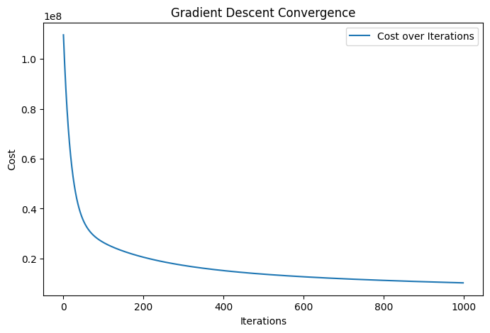
    def plot_cost_history(self):
        """
        Plot the cost history over iterations.
        """
        plt.figure(figsize=(8, 5))
        plt.plot(self.cost_history, label="Cost over Iterations")
        plt.xlabel("Iterations")
        plt.ylabel("Cost")
        plt.title("Gradient Descent Convergence")
        plt.legend()
        plt.show()

# Instantiate the polynomial regression model with degree 2
poly_reg = PolynomialRegression(degree=2, learning_rate=0.001, iterations=1000, scale=True)

# Fit the model using the training data
poly_reg.fit(X_train, y_train)

# Make predictions on the test data
y_pred = poly_reg.predict(X_test)

# Evaluate the model using Mean Squared Error (MSE)
mse = mean_squared_error(y_test, y_pred)
print("Test Mean Squared Error:", mse)

# Plot the cost history to observe convergence
poly_reg.plot_cost_history()

Test Mean Squared Error: 59698053.45753728

Polynomial Regression using scikit-learn

from sklearn.preprocessing import StandardScaler, PolynomialFeatures
from sklearn.linear_model import LinearRegression

# First, manually scale the data using StandardScaler
scaler = StandardScaler()
X_train_scaled = scaler.fit_transform(X_train)
X_test_scaled = scaler.transform(X_test)

# Create polynomial features using scikit-learn
poly_features = PolynomialFeatures(degree=2, include_bias=False)
X_train_poly = poly_features.fit_transform(X_train_scaled)
X_test_poly = poly_features.transform(X_test_scaled)

# Fit a LinearRegression model
lin_reg = LinearRegression()
lin_reg.fit(X_train_poly, y_train)
y_pred_sklearn = lin_reg.predict(X_test_poly)
mse_sklearn = mean_squared_error(y_test, y_pred_sklearn)
print("scikit-learn Polynomial Regression MSE:", mse_sklearn)

scikit-learn Polynomial Regression MSE: 234990527.49339545

from sklearn.metrics import mean_squared_error, mean_absolute_error, r2_score

# Compute error metrics for manual implementation
mse_manual = mean_squared_error(y_test, y_pred)
rmse_manual = np.sqrt(mse_manual)
mae_manual = mean_absolute_error(y_test, y_pred)
r2_manual = r2_score(y_test, y_pred)

# Compute error metrics for scikit-learn implementation
mse_sklearn = mean_squared_error(y_test, y_pred_sklearn)
rmse_sklearn = np.sqrt(mse_sklearn)
mae_sklearn = mean_absolute_error(y_test, y_pred_sklearn)
r2_sklearn = r2_score(y_test, y_pred_sklearn)

# Print results
print("Manual Polynomial Regression:")
print(f"   MSE  : {mse_manual:.4f}")
print(f"   RMSE : {rmse_manual:.4f}")
print(f"   MAE  : {mae_manual:.4f}")
print(f"   R²   : {r2_manual:.4f}")
print("\nScikit-Learn Polynomial Regression:")
print(f"   MSE  : {mse_sklearn:.4f}")
print(f"   RMSE : {rmse_sklearn:.4f}")
print(f"   MAE  : {mae_sklearn:.4f}")
print(f"   R²   : {r2_sklearn:.4f}")

Manual Polynomial Regression:
   MSE  : 59698053.4575
   RMSE : 7726.4515
   MAE  : 4168.0573
   R²   : 0.2301

Scikit-Learn Polynomial Regression:
   MSE  : 234990527.4934
   RMSE : 15329.4008
   MAE  : 7138.0699
   R²   : -2.0305