Implementing Linear Regression for Predicting House Prices (From Scratch)

Introduction

Bellow is my notebook from Kaggle for my project on implementing Linear Regression from scratch for Predicting House Prices and comparing it to scikit-learn predefined one.
Enjoy!

Notebook

# This Python 3 environment comes with many helpful analytics libraries installed
# It is defined by the kaggle/python Docker image: https://github.com/kaggle/docker-python
# For example, here's several helpful packages to load

import numpy as np # linear algebra
import pandas as pd # data processing, CSV file I/O (e.g. pd.read_csv)

# Input data files are available in the read-only "../input/" directory
# For example, running this (by clicking run or pressing Shift+Enter) will list all files under the input directory

import os
for dirname, _, filenames in os.walk('/kaggle/input'):
    for filename in filenames:
        print(os.path.join(dirname, filename))

# You can write up to 20GB to the current directory (/kaggle/working/) that gets preserved as output when you create a version using "Save & Run All" 
# You can also write temporary files to /kaggle/temp/, but they won't be saved outside of the current session

/kaggle/input/the-boston-houseprice-data/boston.csv

Overview

In this notebook i will predict the house prices using linear regression. i will implement everything from scratch then compare my results to a predefined algorithm in scikit learn.

Dataset

first i will load and explore the dataset. i’m working on Boston House Prices on Kaggle

https://www.kaggle.com/datasets/fedesoriano/the-boston-houseprice-data

df = pd.read_csv("/kaggle/input/the-boston-houseprice-data/boston.csv")
df.head()

	CRIM	ZN	INDUS	CHAS	NOX	RM	AGE	DIS	RAD	TAX	PTRATIO	B	LSTAT	MEDV
0	0.00632	18.0	2.31	0	0.538	6.575	65.2	4.0900	1	296.0	15.3	396.90	4.98	24.0
1	0.02731	0.0	7.07	0	0.469	6.421	78.9	4.9671	2	242.0	17.8	396.90	9.14	21.6
2	0.02729	0.0	7.07	0	0.469	7.185	61.1	4.9671	2	242.0	17.8	392.83	4.03	34.7
3	0.03237	0.0	2.18	0	0.458	6.998	45.8	6.0622	3	222.0	18.7	394.63	2.94	33.4
4	0.06905	0.0	2.18	0	0.458	7.147	54.2	6.0622	3	222.0	18.7	396.90	5.33	36.2

df.shape

(506, 14)

df.info()

<class 'pandas.core.frame.DataFrame'>
RangeIndex: 506 entries, 0 to 505
Data columns (total 14 columns):
 #   Column   Non-Null Count  Dtype  
---  ------   --------------  -----  
 0   CRIM     506 non-null    float64
 1   ZN       506 non-null    float64
 2   INDUS    506 non-null    float64
 3   CHAS     506 non-null    int64  
 4   NOX      506 non-null    float64
 5   RM       506 non-null    float64
 6   AGE      506 non-null    float64
 7   DIS      506 non-null    float64
 8   RAD      506 non-null    int64  
 9   TAX      506 non-null    float64
 10  PTRATIO  506 non-null    float64
 11  B        506 non-null    float64
 12  LSTAT    506 non-null    float64
 13  MEDV     506 non-null    float64
dtypes: float64(12), int64(2)
memory usage: 55.5 KB

df.describe()

	CRIM	ZN	INDUS	CHAS	NOX	RM	AGE	DIS	RAD	TAX	PTRATIO	B	LSTAT	MEDV
count	506.000000	506.000000	506.000000	506.000000	506.000000	506.000000	506.000000	506.000000	506.000000	506.000000	506.000000	506.000000	506.000000	506.000000
mean	3.613524	11.363636	11.136779	0.069170	0.554695	6.284634	68.574901	3.795043	9.549407	408.237154	18.455534	356.674032	12.653063	22.532806
std	8.601545	23.322453	6.860353	0.253994	0.115878	0.702617	28.148861	2.105710	8.707259	168.537116	2.164946	91.294864	7.141062	9.197104
min	0.006320	0.000000	0.460000	0.000000	0.385000	3.561000	2.900000	1.129600	1.000000	187.000000	12.600000	0.320000	1.730000	5.000000
25%	0.082045	0.000000	5.190000	0.000000	0.449000	5.885500	45.025000	2.100175	4.000000	279.000000	17.400000	375.377500	6.950000	17.025000
50%	0.256510	0.000000	9.690000	0.000000	0.538000	6.208500	77.500000	3.207450	5.000000	330.000000	19.050000	391.440000	11.360000	21.200000
75%	3.677083	12.500000	18.100000	0.000000	0.624000	6.623500	94.075000	5.188425	24.000000	666.000000	20.200000	396.225000	16.955000	25.000000
max	88.976200	100.000000	27.740000	1.000000	0.871000	8.780000	100.000000	12.126500	24.000000	711.000000	22.000000	396.900000	37.970000	50.000000

# Shuffle the data
data = df.sample(frac=1, random_state=42).reset_index(drop=True)

# Calculate the number of samples for each set
train_size = int(0.7 * len(data))
val_size = int(0.15 * len(data))

# Split the dataset into training, validation, and test sets
train_data = data[:train_size] # training data (70%)
val_data = data[train_size:train_size+val_size] # validation data (15%)
test_data = data[train_size+val_size:] # test data (15%)

# Split the features and target for each set
X_train = train_data.drop('MEDV', axis=1)
y_train = train_data['MEDV']

X_val = val_data.drop('MEDV', axis=1)
y_val = val_data['MEDV']

X_test = test_data.drop('MEDV', axis=1)
y_test = test_data['MEDV']

print(f"Training set size: {len(X_train)} samples")
print(f"Validation set size: {len(X_val)} samples")
print(f"Test set size: {len(X_test)} samples")

Training set size: 354 samples
Validation set size: 75 samples
Test set size: 77 samples

Model

Linear Regression from scratch

class LinearRegression:
    def __init__(self, alpha=0.01, iterations=1000, scale=False):
        self.alpha = alpha  # Learning rate
        self.iterations = iterations  # Number of iterations for gradient descent
        self.scale = scale  # Whether to scale the features or not
        self.w = None  # Weights
        self.b = None  # Bias
        self.cost_history = []  # List to track cost history

    def scale_features(self, X):
        """Scale features using mean and std deviation (standardization)."""
        self.mean = np.mean(X, axis=0)
        self.std = np.std(X, axis=0)
        return (X - self.mean) / self.std

    def fit(self, X, y):
        """Fit the model to the training data using gradient descent."""
        m = len(y)  # Number of training examples
        
        # If scaling is needed, scale the features
        if self.scale:
            X = self.scale_features(X)

        # Initialize weights (w) and bias (b)
        self.w = np.zeros(X.shape[1])
        self.b = 0

        # Perform gradient descent
        for i in range(self.iterations):
            predictions = X.dot(self.w) + self.b
            error = predictions - y

            # Gradient of the cost function with respect to w and b
            dw = (1/m) * np.dot(X.T, error)
            db = (1/m) * np.sum(error)

            # Update weights and bias
            self.w -= self.alpha * dw
            self.b -= self.alpha * db

            # Calculate the cost (Mean Squared Error)
            cost = (1/(2*m)) * np.sum(error ** 2)
            self.cost_history.append(cost)

    def predict(self, X):
        """Make predictions using the trained model."""
        # If scaling was applied, scale the new data as well
        if self.scale:
            X = (X - self.mean) / self.std
        return X.dot(self.w) + self.b

    def get_cost_history(self):
        return self.cost_history

import matplotlib.pyplot as plt

def mean_squared_error(y_true, y_pred):
    m = len(y_true)
    return (1/m) * np.sum((y_true - y_pred) ** 2)

# Initialize and train the model
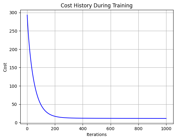
model = LinearRegression(alpha=0.01, iterations=1000, scale=True)
model.fit(X_train, y_train)

cost_history = model.get_cost_history()

plt.plot(range(1, len(cost_history) + 1), cost_history, color='blue')
plt.title('Cost History During Training')
plt.xlabel('Iterations')
plt.ylabel('Cost')
plt.grid(True)
plt.show()

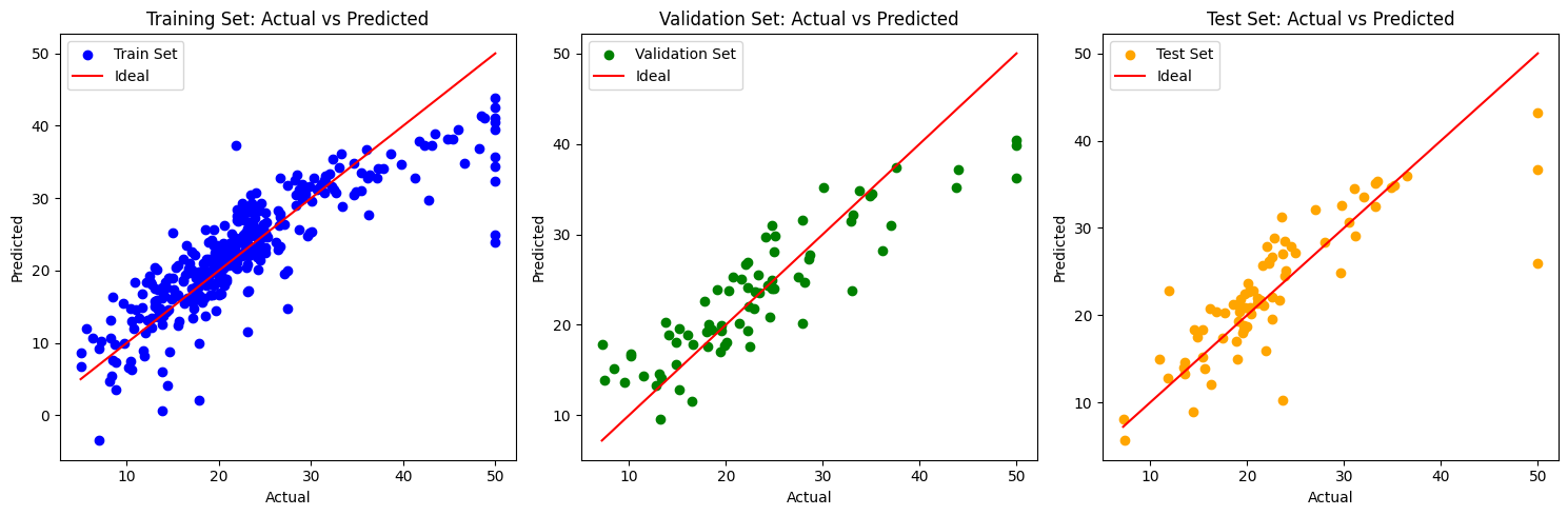
# Make predictions on all datasets
y_train_pred = model.predict(X_train)
y_val_pred = model.predict(X_val)
y_test_pred = model.predict(X_test)

# Calculate Mean Squared Error for all datasets
train_mse = mean_squared_error(y_train, y_train_pred)
val_mse = mean_squared_error(y_val, y_val_pred)
test_mse = mean_squared_error(y_test, y_test_pred)

print(f"Training MSE: {train_mse}")
print(f"Validation MSE: {val_mse}")
print(f"Test MSE: {test_mse}")

Training MSE: 22.384617927405444
Validation MSE: 21.208792092413585
Test MSE: 22.102794782467647

# Plot the actual vs predicted values for all datasets
plt.figure(figsize=(15, 5))

# Training data plot
plt.subplot(1, 3, 1)
plt.scatter(y_train, y_train_pred, color='blue', label="Train Set")
plt.plot([min(y_train), max(y_train)], [min(y_train), max(y_train)], color='red', label="Ideal")
plt.title('Training Set: Actual vs Predicted')
plt.xlabel('Actual')
plt.ylabel('Predicted')
plt.legend()

# Validation data plot
plt.subplot(1, 3, 2)
plt.scatter(y_val, y_val_pred, color='green', label="Validation Set")
plt.plot([min(y_val), max(y_val)], [min(y_val), max(y_val)], color='red', label="Ideal")
plt.title('Validation Set: Actual vs Predicted')
plt.xlabel('Actual')
plt.ylabel('Predicted')
plt.legend()

# Test data plot
plt.subplot(1, 3, 3)
plt.scatter(y_test, y_test_pred, color='orange', label="Test Set")
plt.plot([min(y_test), max(y_test)], [min(y_test), max(y_test)], color='red', label="Ideal")
plt.title('Test Set: Actual vs Predicted')
plt.xlabel('Actual')
plt.ylabel('Predicted')
plt.legend()

plt.tight_layout()
plt.show()

Linear Regression using scikit-learn and comparison

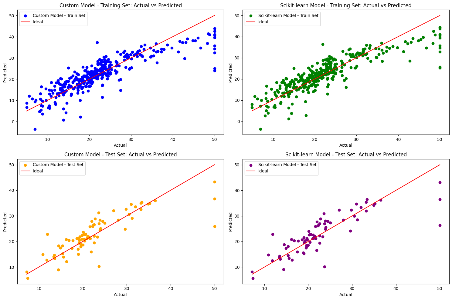
from sklearn.linear_model import LinearRegression as SklearnLR
from sklearn.metrics import mean_squared_error

# Scikit-learn Linear Regression Model
sklearn_model = SklearnLR()
sklearn_model.fit(X_train, y_train)
y_train_pred_sklearn = sklearn_model.predict(X_train)
y_val_pred_sklearn = sklearn_model.predict(X_val)
y_test_pred_sklearn = sklearn_model.predict(X_test)

# Calculate Mean Squared Error for both models
train_mse = mean_squared_error(y_train, y_train_pred)
val_mse = mean_squared_error(y_val, y_val_pred)
test_mse = mean_squared_error(y_test, y_test_pred)

train_mse_sklearn = mean_squared_error(y_train, y_train_pred_sklearn)
val_mse_sklearn = mean_squared_error(y_val, y_val_pred_sklearn)
test_mse_sklearn = mean_squared_error(y_test, y_test_pred_sklearn)

print("Custom Model MSE:")
print(f"Training MSE: {train_mse}")
print(f"Validation MSE: {val_mse}")
print(f"Test MSE: {test_mse}")

print("\nScikit-learn Model MSE:")
print(f"Training MSE: {train_mse_sklearn}")
print(f"Validation MSE: {val_mse_sklearn}")
print(f"Test MSE: {test_mse_sklearn}")

# Plot the actual vs predicted values for both models

plt.figure(figsize=(15, 10))

# Custom Model - Training Data
plt.subplot(2, 2, 1)
plt.scatter(y_train, y_train_pred, color='blue', label="Custom Model - Train Set")
plt.plot([min(y_train), max(y_train)], [min(y_train), max(y_train)], color='red', label="Ideal")
plt.title('Custom Model - Training Set: Actual vs Predicted')
plt.xlabel('Actual')
plt.ylabel('Predicted')
plt.legend()

# Scikit-learn Model - Training Data
plt.subplot(2, 2, 2)
plt.scatter(y_train, y_train_pred_sklearn, color='green', label="Scikit-learn Model - Train Set")
plt.plot([min(y_train), max(y_train)], [min(y_train), max(y_train)], color='red', label="Ideal")
plt.title('Scikit-learn Model - Training Set: Actual vs Predicted')
plt.xlabel('Actual')
plt.ylabel('Predicted')
plt.legend()

# Custom Model - Test Data
plt.subplot(2, 2, 3)
plt.scatter(y_test, y_test_pred, color='orange', label="Custom Model - Test Set")
plt.plot([min(y_test), max(y_test)], [min(y_test), max(y_test)], color='red', label="Ideal")
plt.title('Custom Model - Test Set: Actual vs Predicted')
plt.xlabel('Actual')
plt.ylabel('Predicted')
plt.legend()

# Scikit-learn Model - Test Data
plt.subplot(2, 2, 4)
plt.scatter(y_test, y_test_pred_sklearn, color='purple', label="Scikit-learn Model - Test Set")
plt.plot([min(y_test), max(y_test)], [min(y_test), max(y_test)], color='red', label="Ideal")
plt.title('Scikit-learn Model - Test Set: Actual vs Predicted')
plt.xlabel('Actual')
plt.ylabel('Predicted')
plt.legend()

plt.tight_layout()
plt.show()

Custom Model MSE:
Training MSE: 22.384617927405444
Validation MSE: 21.208792092413585
Test MSE: 22.102794782467647

Scikit-learn Model MSE:
Training MSE: 22.018971306970627
Validation MSE: 22.53291330113675
Test MSE: 22.14619818293375